DistributedArrays.jl
DistributedArrays package provides DArray object that can be split across several processes (set of workers), either on the same or multiple nodes. This allows use of arrays that are too large to fit in memory on one node. Each process operates on the part of the array that it owns – this provides a very natural way to achieve parallelism for large problems.
- Each worker can read any elements using their global indices
- Each worker can write only to the part that it owns $~\Rightarrow~$ automatic parallelism and safe execution
DistributedArrays is not part of the standard
library, so usually you need to install it yourself (it will typically write into ~/.julia/environments/versionNumber
directory):
] add DistributedArrays
We need to load DistributedArrays on every worker:
using Distributed
addprocs(4)
@everywhere using DistributedArrays
n = 10
data = dzeros(Float32, n, n);          # distributed 2D array of 0's
data                                   # can access the entire array
data[1,1], data[n,5]                   # can use global indices
data.dims                              # global dimensions (10, 10)
data[1,1] = 1.0                        # error: cannot write from the control process!
@spawnat 2 data.localpart[1,1] = 1.5   # success: can write locally
data
Let’s check data distribution across workers:
for i in workers()
    @spawnat i println(localindices(data))
end
rows, cols = @fetchfrom 3 localindices(data)
println(rows)     # the rows owned by worker 3
We can only write into data from its “owner” workers using local indices on these workers:
@everywhere function fillLocalBlock(data)
    h, w = localindices(data)
    for iGlobal in h                         # or collect(h)
        iLoc = iGlobal - h.start + 1         # always starts from 1
        for jGlobal in w                     # or collect(w)
            jLoc = jGlobal - w.start + 1     # always starts from 1
            data.localpart[iLoc,jLoc] = iGlobal + jGlobal
        end
    end
end
for i in workers()
    @spawnat i fillLocalBlock(data)
end
data   # now the distributed array is filled
@fetchfrom 3 data.localpart    # stored on worker 3
minimum(data), maximum(data)   # parallel reduction
One-liners to generate distributed arrays:
a = dzeros(100,100,100);      # 100^3 distributed array of 0's
b = dones(100,100,100);       # 100^3 distributed array of 1's
c = drand(100,100,100);       # 100^3 uniform [0,1]
d = drandn(100,100,100);      # 100^3 drawn from a Gaussian distribution
d[1:10,1:10,1]
e = dfill(1.5,100,100,100);   # 100^3 fixed value
You can find more information about the arguments by typing ?DArray. For example, you have a lot of control over the
DArray’s distribution across workers. Before I show the examples, let’s define a convenient function to show the array’s
distribution:
function showDistribution(x::DArray)
    for i in workers()
        @spawnat i println(localindices(x))
    end
end
nworkers()                                  # 4
data = dzeros((100,100), workers()[1:2]);   # define only on the first two workers
showDistribution(data)
square = dzeros((100,100), workers()[1:4], [2,2]);   # 2x2 decomposition
showDistribution(square)
slab = dzeros((100,100), workers()[1:4], [1,4]);   # 1x4 decomposition
showDistribution(slab)
You can take a local array and distribute it across workers:
e = fill(1.5, (10,10))   # local array
de = distribute(e)       # distribute `e` across all workers
showDistribution(de)
Exercise 9
Using either
toporhtopcommand on Cassiopeia, study memory usage with DistributedArrays. Are these arrays really distributed across processes? Use a largish array for this: large enough to spot memory usage, but not too large not to exceed physical memory and not to block other participants (especially if you do this on the login node).
Building a distributed array from local pieces 1
Let’s restart Julia with julia (single control process) and load the packages:
using Distributed
addprocs(4)
using DistributedArrays       # important to load this after addprocs()
@everywhere using LinearAlgebra
We will define an 8x8 matrix with the main diagonal and two off-diagonals (tridiagonal matrix). The lines show our matrix distribution across workers:
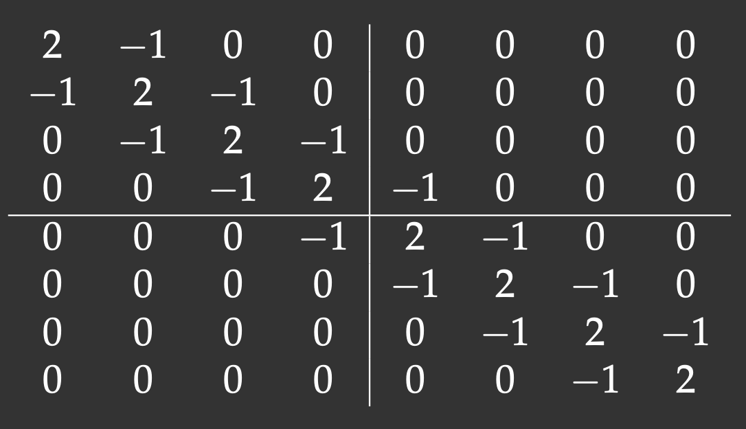
Notice that with the 2x2 decomposition two of the 4 blocks are also tridiagonal matrices. We’ll define a function to initiate them:
@everywhere function tridiagonal(n)
    la = zeros(n,n)
    la[diagind(la,0)] .= 2.   # diagind(la,k) provides indices of the kth diagonal of a matrix
    la[diagind(la,1)] .= -1.
    la[diagind(la,-1)] .= -1.
    return la
end
We also need functions to define the other two blocks:
@everywhere function upperRight(n)
    la = zeros(n,n)
    la[n,1] = -1.
    return la
end
@everywhere function lowerLeft(n)
    la = zeros(n,n)
    la[1,n] = -1.
    return la
end
We use these functions to define local pieces on each block and then create a distributed 8x8 matrix on a 2x2 process grid:
d11 = @spawnat 2 tridiagonal(4)
d12 = @spawnat 3 lowerLeft(4)
d21 = @spawnat 4 upperRight(4)
d22 = @spawnat 5 tridiagonal(4)
d = DArray(reshape([d11 d12 d21 d22],(2,2)))   # create a distributed 8x8 matrix on a 2x2 process grid
d
Exercise 10
At this point, if you redefine
showDistribution()(need to do this only on the control process!), most likely you will see no output if you runshowDistribution(d). Any idea why?
-
This example was adapted from Baolai Ge’s (SHARCNET) presentation. ↩︎