Setup and running Jupyter notebooks
Disclaimer: These notes started few years ago from the official SWC lesson but then evolved quite a bit to include other topics.
| Python pros | Python cons |
|---|---|
| elegant scripting language | slow (interpreted, dynamically typed) |
| powerful, compact constructs for many tasks | |
| very popular across all fields | |
| huge number of external libraries |
Starting Python in a Jupyter notebook
There are many ways to run Python commands:
- from a Unix shell you can start a Python shell and type commands there,
- you launch Python scripts saved in plain text *.py files,
- you can execute Python cells inside Jupyter notebooks; the code is stored inside JSON files, displayed as HTML
Today we will be using a Jupyter notebook. You have several options:
-
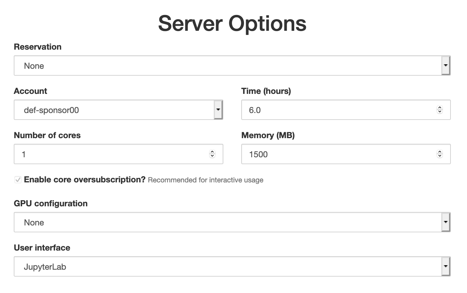
Main option: use JupyterHub on our second training cluster: point your browser to https://uu.c3.ca, log in with yesterday’s username and today’s password, then launch a Jupyter Hub server with time = 6 hours, 1 CPU core, memory = 1500 MB, GPU configuration = None, user interface = JupyterLab
-
Second option: use syzygy.ca with one of the following accounts:
- if you have a university computer ID → go to https://syzygy.ca, under Launch select your institution, then log in with your university credentials
- if you have a Google account → go to https://syzygy.ca, under Launch select either Cybera or PIMS, then log in with your Google account
- if you have a GitHub account → go to https://westgrid.syzygy.ca, sign in with your GitHub account
In either case (1-2) start a new Python 3 notebook.
Note that syzygy.ca is a free community service run on Compute Canada cloud and used heavily for undergraduate teaching, with no uptime guarantees. In other words, it usually works, but it could be unstable or down.
- Third option: if previously in our courses you have used
cassiopeia.c3.cavia SSH, and you remember your username!, you can ssh there and then work in the terminal:
$ source projects/def-sponsor00/shared/astro/bin/activate
$ python
Python 3.7.4 (default, Jul 18 2019, 19:34:02)
[GCC 5.4.0] on linux
Type "help", "copyright", "credits" or "license" for more information.
>>> import numpy as np
Working in the terminal, you won’t have access to all the bells and whistles of the Jupyter interface, and you will have to plot matplotlib graphics into remote PNG files and then download them to view locally on your computer, but it’s doable.
- Local option: finally, the last option for more advanced users, if you have Python + Jupyter installed locally on
your computer, and you know what you are doing, you can start a Jupyter notebook locally from your shell by typing
jupyter notebook. If running locally, for this workshop you will need the following Python packages installed on your computer: numpy, matplotlib, pandas, scikit-image, xarray, nc-time-axis, netcdf4.
Jupyter interface at uu.c3.ca
- File | Save As - to rename your notebook
- File | New Launcher - to open a new launcher dashboard, e.g. to start a terminal
- File | Logout - to terminate your job (everything is running inside a Slurm job!)
Navigating notebook cells
Explain: tab completion, annotating code, displaying figures inside the notebook.
- Esc - leave the cell (border becomes blue) to the control mode
- “A” - insert a cell above the current cell
- “B” - insert a cell below the current cell
- “X” - delete the current cell
- “M” - turn the current cell into the markdown cell
- “H” - to display help
- Enter - re-enter the cell (border becomes green) from the control mode
- can enter Latex equations in a markdown cell, e.g. $int_0^\infty f(x)dx$
print(1/2) # to run all commands in the cell, either use the Run button, or press shift+return